Everyone knows that objects falling under the influene of gravity near the surface of the earth experience constant acceleration of about 32 ft/s^2^, neglecting air resistance. Anyone who has taken elementary physics knows that the speed of a ball after it collides with the floor will be equal to its speed before impact, multiplied by ts coefficident of restitution. The goal; of the experiment was to use the Matlab image processing toolbox to verify both these statements.
This is of a very crude way to do this. The main point of the assignment was to use these questions as a way to teach ourselves how to use the image processing toolbox to answer scientific questions and test hypotheses. If you really want to measure gravitational acceleration accurately with simple tools, you should use the Kater pendulum.
In this video, we show footage at 15 frames/sec of a capstone student bouncing a ball in a gym at NJIT. We analysze this using the Matlab pendulum demonstration as a guide. First we select a rectangle in the middle of the picture where the ball is is bouncing. We convert the image from RGB to grayscale (2nd column), threshhold the image (i.e. reduce from grayscale to black & white) and follow the location of the largest spot after threshholding (third column).
This was surprisingly easy to do. There was one small hiccup. After converting from RGB to greyscale, we found that there was insufficient contrast between the blue ball and the white wall behind it, and after the threshholding, an image analysis subroutine often failed to identify the ball as the largest object in the figure, especially when the ball was near the floor. This was solved by first converting the image from RGB to HSV (hue-saturation-value coordinates, sort of like cylindrical coordinates for colors). By looking at the hue channel, the blue ball became very easy to spot. The second column in the movie above shows the coordinate.
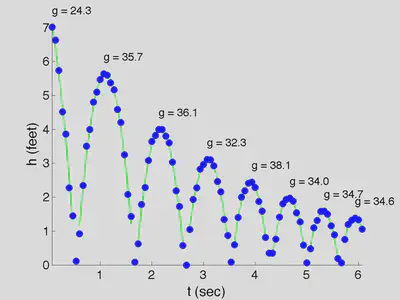
We can find center of mass of the largest spot (the red star), plot its $y$-coordinate as a function of time (blue spots below), and fit each trajectory to a parabola (green lines below). The coefficient of the $t^2$ term in each parabola is equal to half the acceleration. On some flights, g is computed near 32 ft/s^2^. On others it is not.
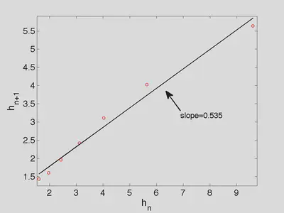
The height a ball reaches on a given bounce is proportional to the velocity at which it leaves the ground. Therefore, we plot the maximum height on flights 2-8 as a function of the maximum height on flights 1-7 and find that the slope, and thus the coefficient of restitution is 0.535.